The Challenge
My fantasy football league had a fun way to determine our draft order: the person who most accurately guesses the amount of runs scored in all seventeen MLB games on Saturday, September 2nd gets to choose their draft position. The worse your guess, the worse your draft position. We had a wide variety of techniques from total guessing to some statistical modeling, and I thought this would be a good chance to think of each of these modeling practices.
The Data
I think baseball barely edges out bowling and darts in entertainment value. The data availability in baseball, however, is awesome! Retrosheets provides game logs in csv format for every game since 1871, and we’re able to import this into R pretty easily. The csv provides no column names, but there is a pretty good data dictionary that tells you what field is what.
In this step, we’ll the data and separate it into two samples: training_game_log is the record of all games before September 2nd in the 2017 season and validation_game_log is the record of the games on September 2nd 2017.
game_log_raw <- read.csv(url("https://raw.githubusercontent.com/andrewnguyen42/raw-data/master/GL2017.TXT"), header = F)

game_log <- game_log_raw %>%
  rename(date = V1
         ,visiting_team = V4
         ,home_team = V7
         ,visiting_score = V10
         ,home_score = V11
         ,visiting_team_earned_runs = V41
         ,home_team_earned_runs = V69
         ,outs_played = V12)%>%
  select(date
         ,visiting_team
         ,home_team
         ,visiting_score
         ,home_score
         ,visiting_team_earned_runs
         ,home_team_earned_runs
         ,outs_played) %>%
  mutate(date = ymd(date)
         ,total_score = visiting_score + home_score)

training_game_log <- game_log %>% filter(date < ymd('2017/09/02'))
validation_game_log <- game_log %>% filter(date == ymd('2017/09/02'))
Model 1: Simple Averages
The first model is really easy. We’ll simply take the average number of runs per game, and then multiply it by the number of games on September 2nd (17).
And yes, this is a totally valid model. Models may be as simple as just guessing the average!
avg_total_score <- training_game_log %>% .$total_score %>% mean
guess_runs <- avg_total_score * nrow(validation_game_log)
actual_runs <- validation_game_log$total_score %>% sum
The actual value is 183 while we guessed 158.2249. In a vacuum, this seems like an okay guess. The games we were interested in, the scoring average was 10.7647 so our average 1.4574 too low for every game.
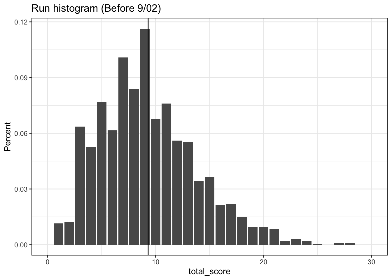
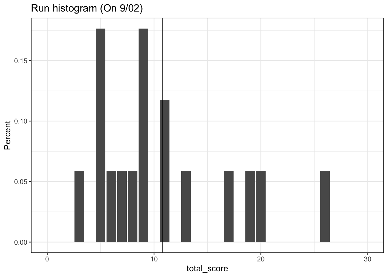
The first histogram is telling of our problem. The total runs has a very heavy skew towards the right, and the mean simply isn’t doing a good job of capturing these outliers. By examining the histogram of the scores on the day-of, we see that the one really high scoring game between the Houston Astros and the Chicago Cubs really throws our prediction off.
This begs the question: how much can we trust the average? After all, the average is a statistic that must be estimated. And since the average is an estimated statistic, we can build confidence intervals around this estimate using t.test. Welch’s t-test is a test to measure how confident the average isn’t 0. Along with the sample average, two other quantities come along for the ride: an upper and lower bound of the average. By using the upper and lower bounds as our average, we can build a range of total runs that we are “confident” that any guess will fall into.
t_test_result <- t.test(training_game_log$total_score)
avg_lower_bound <- t_test_result$conf.int[1]
avg_upper_bound <- t_test_result$conf.int[2]

lower_guess <- avg_lower_bound * nrow(validation_game_log)
upper_guess <- avg_upper_bound * nrow(validation_game_log)
Our lower bound if 154.8664 and our upper bound is 161.5835, but the actual value is 183! In this case, our model is way off.
One important technical note is that Welch’s t-test relies on our data being normally distributed. Looking at the graph, it’s pretty clear that the data is skewed and runs are not normally distributed (a call to jarque.bera.test will confirm this).
Maybe this model isn’t perfect, but what is good about it? It’s really simple, understandable, and we have a way to say that our prediction was crappy. Further, I suspect that in the long run, this may actually be the correct model (more on this in another post).
Okay, so maybe if we try a more statistically robust model, we can remedy what ills us.
Model 2: The Bootstrap
The fatal flaw of our last model is that our guess relies a lot on underlying distribution of runs to be normal. We can solve this with a popular simulation technique called bootstrapping.
Bootstrapping is a general purpose technique for estimating a quantity without assuming anything about the underlying distribution. This is really nice for our purpose. The formula for the bootstrap is as follows:
- Draw a subset of our data with replacement
- Calculate the quantity of interest on that subset
- Repeat steps 1-2
ntimes and save each calculation - We now have a distribution of the quantity of interest
Using this distribution of data, we can take averages of our quantity of interest and do inference!
We can use the bootstrap to make a guess at any property of our underlying data, for example we could use the bootstrap to guess the average and build confidence-intervals without assuming the underlying distribution. However, let’s try to estimate the 17-game total number of runs directly!
set.seed(1)

bootstrap_samples <- replicate(n = 1000
                    , expr = training_game_log$total_score %>%
                      sample(size = nrow(validation_game_log), replace = TRUE))

bootstrap_sums <- bootstrap_samples %>% apply(2, sum)
bootstrap_guess <- bootstrap_sums %>% mean
Here, we have done something subtle that I want to be really explicit about. Instead of building a distribution of single game totals, we have built a distribution of 17-game totals using the bootstrap. The bootstrap forumla above would go like this:
- Draw 17 random games with replacement (done with
sampleandreplace) - Calculate the total runs for those 17 games (
sum) - Repeat steps 1-2
1000times and save each calculation (replicate) - We now have a distribution of the quantity of interest (save in
data.frame)
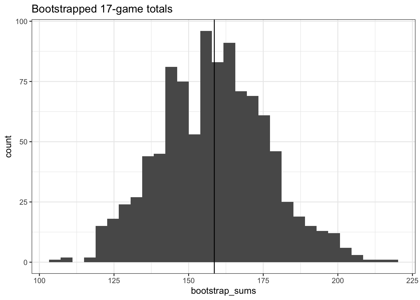
If we take the average of this distribution, our guess is still only 158.609 vs the actual seventeen-game sum of 183. This doesn’t appear much better than our guess of just averages, but what about our confidence interval? According to this some bootstrapping theory, we can estimate an upper and lower bound via the following process:
- Calculate the sum for each of our bootstrap samples, there will be 1000 of these
- Subtract out our average estimate
bootstrap_guessfrom each sum, this gives us a list of how far awaybootstrap_guesswas from each bootstrap sample - Rank order our bootstrap errors
- The lower bound is
bootstrap_guess+ the 5th percentile bootstrap error - The upper bound is
bootstrap_guess+ the 95th percentile bootstrap error
bootstrap_errors <- bootstrap_sums - bootstrap_guess
bootstrap_lb <- bootstrap_guess + quantile(bootstrap_errors, .05)
bootstrap_ub <- bootstrap_guess + quantile(bootstrap_errors, .95)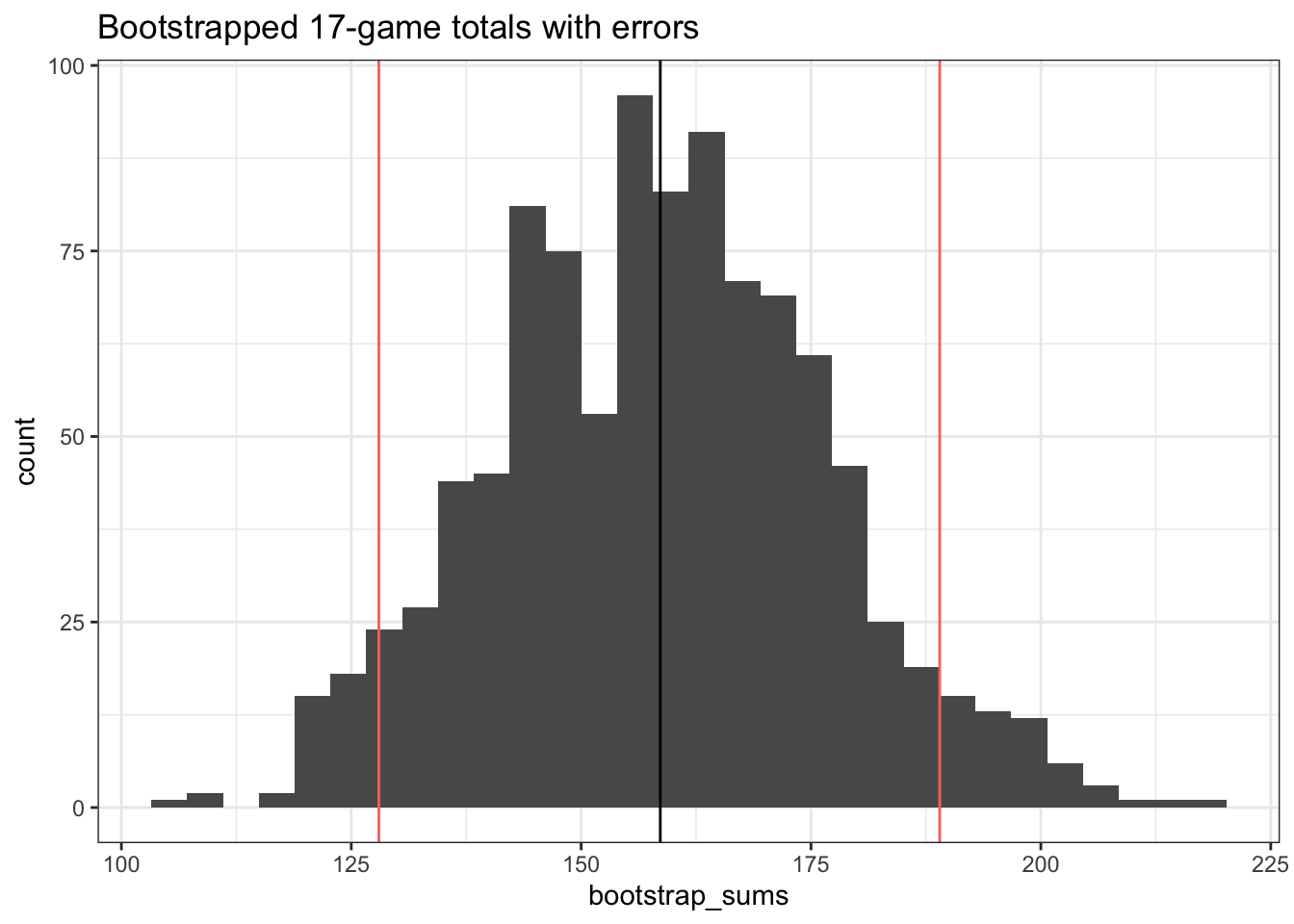
Sweet! Our actual_runs of 183 falls within our confidence interval of 128 and 189.
So what was good about this model? Our confidence intervals were able to more accurately capture how uncertain the number of runs is. This is because we didn’t rely on the underlying distribution of our data to be normally distributed, and we relied on the data to tell us about its uncertainty.
What was bad about this model? Although we are happy that actual_runs fell within our confidence interval, the average guess was still kind of crappy. This is the model I chose, and I ended up losing the challenge. In our next model, we’ll try to guess closer to the actual value.
Model 3: A more specific model
It has become clear that fancier computation isn’t helping us guess a better average. Thankfully, we have more and different data than just run totals. We have the sense that some teams are way better at offense or defense than others. Our previous two models were simply ignoring this fact when they took a simple average or used a simulation with every team included in it. For this model, we’ll use the fact that we know what teams are playing in our seventeen game lineup and that we also know how many runs their defense allows.
Earned runs is a measure of how many runs a defense allows without the aid of mistakes like walks or errors. By constructing an per-nine-inning average of the earned runs by a team, we can add up the team earned run average (TERA) for all twenty-four teams in our seventeen game set. We hope that this will capture the quality of defenses in our model and give us a better estimate.
earned_runs_average <- earned_runs %>%
  group_by(team) %>%
  summarise(era = 9*sum(earned_runs)/sum(innings_pitched))

ERA_guess <- validation_game_log  %>%
  inner_join(earned_runs_average, by = c("home_team"="team")) %>%
  inner_join(earned_runs_average, by = c("visiting_team"="team"), suffix = c('_home','_visiting')) %>%
  mutate(total_era = era_visiting + era_home) %>%
  .$total_era %>%
  sum
Using this technique, we get a kind of paltry 147.0271. Sigh a guess that’s even worse than just guessing the average. We can see what went wrong in our histogram.
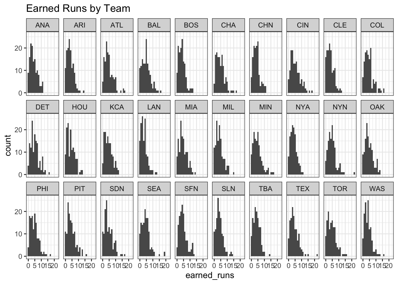
Again, our earned runs distribution is highly non-normal. So maybe our choice of the average is bad and we need to (you guessed it) bootstrap our average. This bootstrap technique will be slightly different from before. Whereas before we bootstrapped averages using the entire sample of teams, we will run a bootstrap for every single team.
- For each team:
- Draw 135 random games with replacement (this is roughly the amount of games in our training sample)
- Calculate the ERA for those 135 games
- Repeat steps 1-2
1000times and save each calculation (replicate) - We now have a distribution of ERA
- Our guess at ERA is the average of that the bootstrap distribution for each team
set.seed(1)

ERA_bootstrap_df <- earned_runs %>%
  split(.$team) %>% #split into a list of dataframes for each team
  map_dbl( function(x) {
    replicate(n = 1000
              , expr = x$earned_runs %>%
                sample(size = 135, replace = TRUE)) %>% mean
    }) %>%
  data.frame(earned_runs_bootstrap = .) %>% rownames_to_column("team")

ERA_bootstrap_guess <- validation_game_log  %>%
  inner_join(ERA_bootstrap_df, by = c("home_team"="team")) %>%
  inner_join(ERA_bootstrap_df, by = c("visiting_team"="team"), suffix = c('_home','_visiting'))%>%
  mutate(total_tera = earned_runs_bootstrap_visiting + earned_runs_bootstrap_home) %>%
  .$total_tera %>%
  sum
It turns out, this was our worst guess yet. At 145.5153 is even worse than our ERA guess and just guessing the average. By comparing the bootstrapped ERA with the calculated ‘vanilla’ ERA, the differences in the guess is really small and the bootstrap ERA ends up being smaller on average.
| team | era | earned_runs_bootstrap |
|---|---|---|
| ANA | 4.15 | 4.11 |
| ARI | 3.65 | 3.62 |
| ATL | 4.72 | 4.68 |
| BAL | 4.81 | 4.76 |
| BOS | 3.69 | 3.7 |
| CHA | 4.83 | 4.7 |
But why does this model fail? Let’s evaluate ERA as a predictor using the bootstrap by building a confidence interval around each team’s ERA.
set.seed(1)
ERA_errors_bootstrap_df <- earned_runs %>%
  split(.$team) %>% #split into a list of dataframes for each team
  map( function(x) { #calculate bootstrap errors for each team
    bootstrap_samples <- replicate(n = 1000
              , expr = x$earned_runs %>% sample(size = 135, replace = TRUE))
    bootstrap_mean <- bootstrap_samples %>% mean
    bootstrap_errors <- bootstrap_samples - bootstrap_mean
    bootstrap_errors
    }) %>% map(function(x) {c(q05 = quantile(x,.05), q95 = quantile(x,.95)) }) %>%
    data.frame %>% t() %>% data.frame %>% rownames_to_column('team') %>%
    rename(lower_se = q05.5., upper_se = q95.95.) %>%
    inner_join(ERA_bootstrap_df) %>%
    mutate(lower_bound = earned_runs_bootstrap + lower_se, upper_bound = earned_runs_bootstrap + upper_se) %>%
select(team, lower_bound, upper_bound)| team | era | lower_bound | upper_bound |
|---|---|---|---|
| ANA | 4.15 | 0 | 10 |
| ARI | 3.65 | 0 | 8 |
| ATL | 4.72 | 1 | 10 |
| BAL | 4.81 | 0 | 11 |
| BOS | 3.69 | 0 | 9 |
| CHA | 4.83 | 1 | 10 |
This table gives the reason for the ERA model’s failure. When we use ERA as a predictor, the range of our prediction is extremely wide. Despite our large sample size, we have almost no confidence in what the actual ERA is for most teams. One thing to note is that the winning model was a variant of this that added up the starting pitcher’s ERA, but individual pitching data was not available on retrosheets.
The model I chose didn’t end up winning the contest and we ended up building some bad models that made bad guesses. But to quote Ta-Nehisi Coates, “This story began, as all writing must, in failure.” There are more improvements to make and more standards to be judged on.
The next really obvious thing is that we only tested our models on one game. Model performance depends on our ability to make a lot of predictions. In my next post I’ll evaluate these models on more games and different time slices.